Neural Networks

In our journey through MLIR and modern compiler technology, we've explored how to build efficient systems for numerical computation. Now, we turn our attention to one of the most important applications of these systems: deep learning. Before diving into how MLIR can optimize neural network computations, it's crucial to understand how neural networks work from first principles.

This section presents a ground-up implementation of a neural network library in pure Python. While this implementation prioritizes clarity over performance, it serves as an excellent foundation for understanding the optimizations that MLIR can provide. By building everything from scratch, we'll gain deep insights into:

The mathematical foundations of neural networks
How automatic differentiation enables learning
The computational patterns that make neural networks ideal for hardware acceleration
Why frameworks like PyTorch and TensorFlow are structured the way they are

In later sections, we'll transform this simple implementation into highly optimized CUDA kernels using MLIR. This progression from a clear but naive implementation to a high-performance compiled version will demonstrate the power of modern compiler technology in deep learning.

The complete source code for this section is available in a separate repository for reference.

Neural networks are everywhere these days, I won't explain too much about why they're useful but if you've used any of the popular libraries like Jax, PyTorch, or TensorFlow, you know they make it easy to build and train complex models. Understanding how these frameworks work under the hood is invaluable. In this section, we'll build a very minimal neural network library from first principles, providing insight into the core mechanisms that power modern deep learning.

Gradients and Optimization

At the heart of neural network training lies the concept of gradients. Think of a gradient as a compass that points in the direction of steepest increase for a function. For a function with multiple inputs $f(x_1, x_2, ..., x_n)$, the gradient $\nabla f$ is a vector containing the rate of change in each direction:

$$\nabla f = \begin{bmatrix}
\frac{\partial f}{\partial x_1} \
\frac{\partial f}{\partial x_2} \
\vdots \
\frac{\partial f}{\partial x_n}
\end{bmatrix}$$

Each component $\frac{\partial f}{\partial x_i}$ tells us how much the function would change if we slightly adjusted that input while keeping all others constant. This information is crucial for training neural networks.

In neural network training, we want to minimize a loss function $L(\theta)$ that measures how well our model performs. The parameters $\theta$ include all the weights and biases in the network - often thousands or millions of values. The gradient $\nabla L(\theta)$ tells us how to adjust each parameter to reduce the loss:

$$
\theta_{t+1} = \theta_t - \alpha \nabla L(\theta_t)
$$

This is gradient descent in action: we repeatedly take small steps (controlled by the learning rate $\alpha$) in the direction opposite to the gradient, gradually finding parameter values that minimize the loss.

Computing these gradients efficiently is crucial. While we could use numerical approximations:

$$
\frac{\partial f}{\partial x_i} \approx \frac{f(x + h\mathbf{e}_i) - f(x)}{h}
$$

where $h$ is a small number and $\mathbf{e}_i$ is the unit vector in direction $i$, this approach is both slow and numerically unstable. Instead, we use automatic differentiation, which computes exact gradients by systematically applying the chain rule through a computation graph.

The chain rule states that for composite functions, derivatives multiply:

$$
\frac{d}{dx}(f(g(x))) = f'(g(x)) \cdot g'(x)
$$

In higher dimensions, this becomes:

$$
\frac{\partial f}{\partial x_i} = \sum_j \frac{\partial f}{\partial y_j} \frac{\partial y_j}{\partial x_i}
$$

where $y_j$ are intermediate values in our computation. This is the foundation of backpropagation, which we'll implement in our neural network library.

Neural Network Theory

A neural network is fundamentally a function that learns to map inputs to outputs through a series of adjustable transformations. The basic building block is the artificial neuron, which mimics how biological neurons process information:

It receives multiple input signals ($x_1, x_2, ..., x_n$)
Each input is weighted by a strength parameter ($w_1, w_2, ..., w_n$)
The weighted inputs are summed together with a bias term ($b$)
The result is passed through an activation function ($\sigma$)

Mathematically, this process is described as:

$$
z = \sum_{i=1}^{n} w_i x_i + b
$$

$$
a = \sigma(z)
$$

where $z$ is the weighted sum (often called the pre-activation), and $a$ is the neuron's output (or activation).

Multiple neurons are organized into layers, and layers are stacked to form a network. In a fully-connected feed-forward neural network, each neuron connects to every neuron in the next layer. For a layer $l$, we can write this compactly in matrix form:

$$
\mathbf{Z}^{[l]} = \mathbf{W}^{[l]} \mathbf{A}^{[l-1]} + \mathbf{b}^{[l]}
$$
$$
\mathbf{A}^{[l]} = \sigma(\mathbf{Z}^{[l]})
$$

where:

$\mathbf{W}^{[l]}$ is the weight matrix for layer $l$
$\mathbf{A}^{[l-1]}$ contains the activations from the previous layer
$\mathbf{b}^{[l]}$ is the bias vector
$\sigma$ applies the activation function to each element

The choice of activation function is crucial as it introduces non-linearity that allows the network to learn complex patterns. Without non-linearity, a neural network would behave like a linear model, regardless of the number of layers it has. This is because the composition of linear functions is still a linear function. Non-linear activation functions enable the network to approximate complex functions and capture intricate relationships in the data. They allow the model to learn from errors and adjust weights in a way that can represent a wider variety of functions. Common choices of activation functions are:

ReLU (Rectified Linear Unit): $\sigma(z) = \max(0, z)$
- Simple and computationally efficient
- Helps prevent vanishing gradients
- Most widely used in modern networks
Sigmoid: $\sigma(z) = \frac{1}{1 + e^{-z}}$
- Squashes values to range [0,1]
- Historically popular but prone to vanishing gradients
- Still useful for binary classification
Tanh: $\sigma(z) = \tanh(z) = \frac{e^z - e^{-z}}{e^z + e^{-z}}$
- Similar to sigmoid but ranges [-1,1]
- Often performs better than sigmoid
- Still can suffer from vanishing gradients
SwiGLU: $\sigma(z) = \text{ReLU}(zW_1 + b_1)V + b_2$
- Introduced in the GLU (Gated Linear Unit) family
- Often used in the Transformer architecture
- Provides a balance between non-linearity and computational efficiency

SwiGLU has become the default choice in many modern networks. I won't go into the details of the GLU family here, but if you're interested in learning more, I recommend checking out the GLU paper. For our purposes, we'll use ReLU as our activation function because it's simpler.

Automatic Differentiation

Automatic differentiation is the engine that powers neural network learning. Unlike numerical differentiation (which approximates derivatives) or symbolic differentiation (which manipulates mathematical expressions), automatic differentiation computes exact derivatives by tracking operations in a computation graph.

Our implementation centers on the Value class, which wraps a scalar value and records the operations performed on it:

class Value:
    def __init__(self, data, _children=(), _op="", label=""):
        self.data = data
        self.grad = 0.0
        self.label = label
        self._backward = lambda: None
        self._prev = set(_children)
        self._op = _op

Each operation (like addition or multiplication) creates a new Value and defines how gradients should flow backward. For example, here's how addition works:

def __add__(self, other):
    other = other if isinstance(other, Value) else Value(other)
    out = Value(self.data + other.data, (self, other), "+")

    def _backward():
        # The gradient flows equally to both inputs
        self.grad += out.grad
        other.grad += out.grad

    out._backward = _backward
    return out

For multiplication, the gradient follows the product rule - each input's gradient is scaled by the other input's value:

def __mul__(self, other):
    other = other if isinstance(other, Value) else Value(other)
    out = Value(self.data * other.data, (self, other), "*")

    def _backward():
        # Each input's gradient is scaled by the other's value
        self.grad += other.data * out.grad
        other.grad += self.data * out.grad

    out._backward = _backward
    return out

The backward pass is initiated by calling backward(), which:

Performs a topological sort of the computation graph
Sets the gradient of the output to 1.0
Propagates gradients backward through the graph

def backward(self):
    # Sort nodes in topological order
    topo = []
    visited = set()

    def topo_sort(v):
        if v not in visited:
            visited.add(v)
            for child in v._prev:
                topo_sort(child)
            topo.append(v)

    topo_sort(self)

    # Backpropagate gradients
    self.grad = 1
    for v in reversed(topo):
        v._backward()

To see this in action, let's create a simple computation graph for the expression relu(a * b + c):

# Create input values
a = Value(2.0, label="a")
b = Value(-3.0, label="b")
c = Value(10.0, label="c")

# Build computation graph
d = a * b
d.label = "d"
e = d + c
e.label = "e"
f = e.relu()
f.label = "f"

Now we can compute the gradients of the output with respect to each input:

print("Gradients after backward pass:")
print(f"a.grad = {a.grad}")
print(f"b.grad = {b.grad}")
print(f"c.grad = {c.grad}")
print(f"d.grad = {d.grad}")
print(f"e.grad = {e.grad}")
print(f"f.grad = {f.grad}")

The resulting computation graph is shown in Figure 1. Each node represents a value, and edges show how values are combined through operations. When we call f.backward(), gradients flow backward through this graph, allowing us to compute how each input affects the final output.

Computation Graph Visualization
Figure 1: Visualization of a computation graph showing how operations are connected and gradients flow backward.

Backpropagation

Backpropagation is the algorithm that enables neural networks to learn from data by efficiently computing gradients of the loss function with respect to the network parameters. It applies the chain rule of calculus to propagate error gradients backward through the network, from the output layer to the input layer.

The process begins with a forward pass, where input data is fed through the network to produce predictions. The loss function $L$ quantifies the difference between these predictions and the true target values. For a mean squared error loss, this is:

$$
L = \frac{1}{n} \sum_{i=1}^{n} (y_i - \hat{y}_i)^2
$$

where $y_i$ are the true values and $\hat{y}_i$ are the predicted values.

The goal of training is to minimize this loss by adjusting the network parameters (weights and biases). This requires computing the gradient of the loss with respect to each parameter:

$$
\frac{\partial L}{\partial w_{ij}^{[l]}}
\text{ and }
\frac{\partial L}{\partial b_i^{[l]}}
$$

for each weight $w_{ij}^{[l]}$ and bias $b_i^{[l]}$ in layer $l$.

Backpropagation computes these gradients efficiently by working backward through the network. For the output layer $L$, we first compute the error term:

$$
\delta^{[L]} = \nabla_a L \odot \sigma'(z^{[L]})
$$

where $\nabla_a L$ is the gradient of the loss with respect to the output activations, $\sigma'(z^{[L]})$ is the derivative of the activation function evaluated at the pre-activation values $z^{[L]}$, and $\odot$ denotes element-wise multiplication.

For hidden layers, the error term is computed recursively:

$$
\delta^{[l]} = ((w^{[l+1]})^T \delta^{[l+1]}) \odot \sigma'(z^{[l]})
$$

where $(w^{[l+1]})^T$ is the transpose of the weight matrix for layer $l+1$.

Finally, the gradients of the loss with respect to the parameters are:

$$
\frac{\partial L}{\partial w_{ij}^{[l]}} = a_j^{[l-1]} \delta_i^{[l]}
$$

$$
\frac{\partial L}{\partial b_i^{[l]}} = \delta_i^{[l]}
$$

where $a_j^{[l-1]}$ is the activation of neuron $j$ in layer $l-1$.

In our implementation, these calculations are handled automatically by the Value class and its operations. When we call loss.backward(), the gradients are computed and stored in the grad attribute of each parameter.

Building Neural Network Components

With our automatic differentiation engine in place, we can build neural network components. The Module class serves as the base for all neural network modules:

class Module:
    """Base class for all neural network modules."""

    def zero_grad(self):
        """Sets gradients of all parameters to zero."""
        for p in self.parameters():
            p.grad = 0

    def parameters(self):
        """Returns a list of all parameters in the module."""
        return []

The Neuron class implements a single neuron that computes a weighted sum of inputs plus a bias, optionally followed by a non-linear activation function:

class Neuron(Module):
    """A single neuron with multiple inputs and one output."""

    def __init__(self, nin, nonlin=True):
        self.w = [Value(random.uniform(-1, 1)) for _ in range(nin)]
        self.b = Value(0)
        self.nonlin = nonlin

    def __call__(self, x):
        act = sum((wi * xi for wi, xi in zip(self.w, x)), self.b)
        return act.relu() if self.nonlin else act

    def parameters(self):
        return self.w + [self.b]

The Layer class groups neurons together to process inputs in parallel:

class Layer(Module):
    """A layer of neurons, where each neuron has the same number of inputs."""

    def __init__(self, nin, nout, **kwargs):
        self.neurons = [Neuron(nin, **kwargs) for _ in range(nout)]

    def __call__(self, x):
        out = [n(x) for n in self.neurons]
        return out[0] if len(out) == 1 else out

    def parameters(self):
        return [p for n in self.neurons for p in n.parameters()]

Finally, the MLP (Multi-Layer Perceptron) class combines layers into a complete network:

class MLP(Module):
    """Multi-layer perceptron (fully connected feed-forward neural network)."""

    def __init__(self, nin, nouts):
        sz = [nin] + nouts
        self.layers = [
            Layer(sz[i], sz[i + 1], nonlin=i != len(nouts) - 1)
            for i in range(len(nouts))
        ]

    def __call__(self, x):
        for layer in self.layers:
            x = layer(x)
        return x

    def parameters(self):
        return [p for layer in self.layers for p in layer.parameters()]

This modular design makes it easy to create networks of any size. For example, a small network for binary classification might look like:

# Create a network with:
# - 2 input features
# - 8 neurons in first hidden layer
# - 8 neurons in second hidden layer
# - 1 output neuron
model = MLP(nin=2, nouts=[8, 8, 1])

The architecture is visualized in Figure 2, showing how neurons are organized into layers and layers are connected to form the complete network.

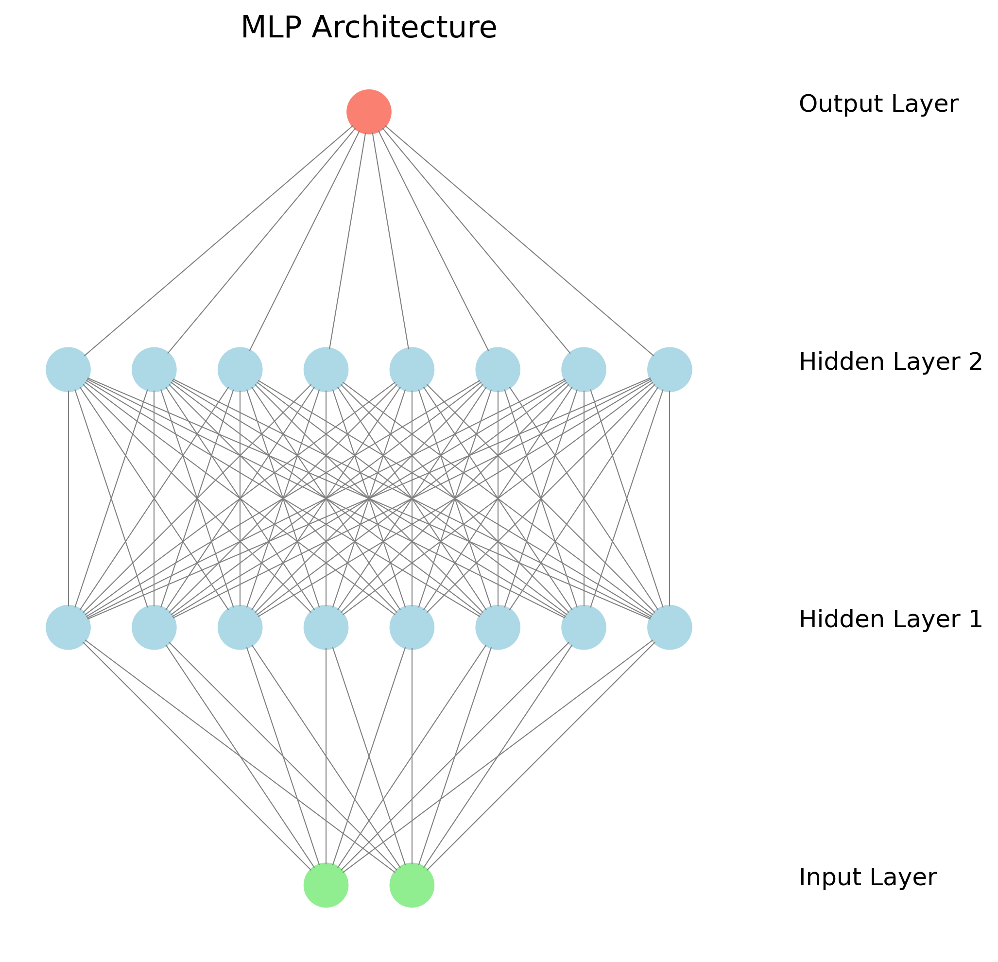
Figure 2: Visualization of our neural network architecture showing multiple layers of neurons.

We can create deeper networks by adding more layers, as shown in Figure 3. Each additional layer allows the network to learn more complex features. Early layers typically learn simple patterns (like edges in images), while deeper layers combine these to recognize more complex patterns (like objects or concepts).

Neural Network Architecture
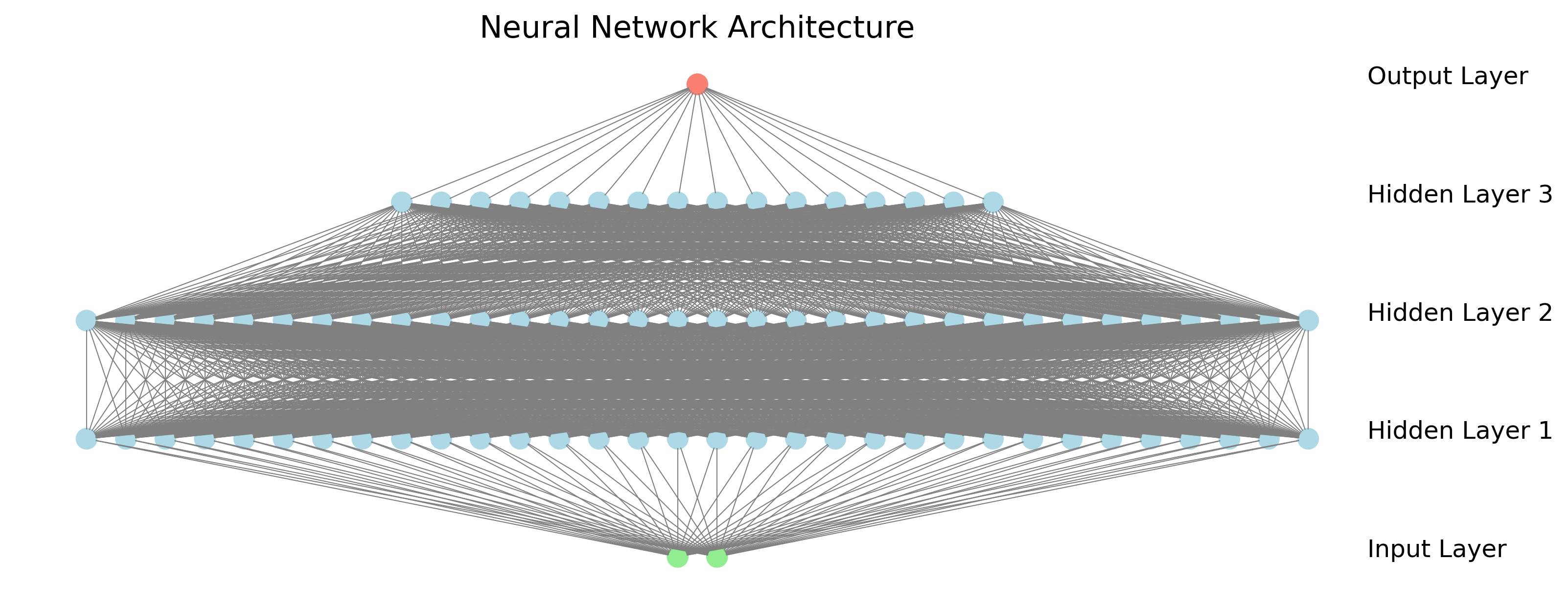
Figure 3: A deeper neural network with multiple hidden layers, showing how layers can be stacked to increase model capacity.

Optimization and Training

To train our neural network, we need an optimizer that updates parameters based on gradients. Our SGD (Stochastic Gradient Descent) optimizer is remarkably simple:

class SGD:
    """
    Stochastic Gradient Descent optimizer.
    """

    def __init__(self, parameters, lr=0.01):
        self.parameters = parameters
        self.lr = lr

    def zero_grad(self):
        """Set all parameter gradients to zero."""
        for p in self.parameters:
            p.grad = 0

    def step(self):
        """
        Updates each parameter as: p = p - lr * p.grad
        """
        for p in self.parameters:
            p.data -= self.lr * p.grad

The optimizer stores references to model parameters, provides a method to zero gradients before each forward pass, and updates parameters using the gradient descent rule:

$$
\theta_{t+1} = \theta_t - \alpha \nabla_\theta L(\theta_t)
$$

where $\theta$ represents the parameters, $\alpha$ is the learning rate, and $\nabla_\theta L(\theta_t)$ is the gradient of the loss function with respect to the parameters.

While more sophisticated optimizers like Adam or RMSProp offer better convergence properties by adapting the learning rate for each parameter based on historical gradient information, SGD illustrates the core principle of gradient-based optimization.

The training process is encapsulated in the Trainer class, which handles data batching, forward and backward passes, parameter updates, and metric tracking:

import random
import matplotlib.pyplot as plt
from tinynn.engine import Value


class Trainer:
    def __init__(self, model, optimizer, loss_fn=None):
        self.model = model
        self.optimizer = optimizer
        self.loss_fn = loss_fn or self._mse_loss

        # Training history
        self.losses = []
        self.accuracies = []

    def _mse_loss(self, pred, target):
        """Mean squared error loss function."""
        return (pred - target) * (pred - target)

    def train(
        self, X, y, n_epochs=100, batch_size=32, verbose=True, early_stopping=True
    ):
        """
        Train the model on the given dataset.

        Args:
            X: Features (list or numpy array)
            y: Target values (list or numpy array)
            n_epochs: Number of training epochs
            batch_size: Mini-batch size
            verbose: Whether to print progress
            early_stopping: Whether to stop early on perfect accuracy

        Returns:
            Dictionary containing training history
        """
        print("Training neural network...")

        for epoch in range(n_epochs):
            # Track metrics for this epoch
            total_loss = 0.0
            correct = 0

            # Shuffle the data
            indices = list(range(len(X)))
            random.shuffle(indices)

            # Mini-batch training
            for start_idx in range(0, len(X), batch_size):
                end_idx = min(start_idx + batch_size, len(X))
                batch_indices = indices[start_idx:end_idx]

                # Zero gradients
                self.optimizer.zero_grad()

                # Accumulate loss and accuracy over the batch
                batch_loss = Value(0.0)

                for idx in batch_indices:
                    # Convert numpy features to Value objects
                    x_vals = [Value(X[idx][0]), Value(X[idx][1])]

                    # Forward pass
                    pred = self.model(x_vals)
                    pred_value = pred[0] if isinstance(pred, list) else pred

                    # Binary cross-entropy loss with tanh activation
                    target = 1.0 if y[idx] == 1 else -1.0  # Use -1/1 targets for tanh

                    # Calculate loss
                    loss = self.loss_fn(pred_value, target)

                    # Accumulate loss
                    batch_loss = batch_loss + loss

                    # Check accuracy
                    pred_class = 1 if pred_value.data > 0 else 0
                    if pred_class == y[idx]:
                        correct += 1

                # Scale loss by batch size
                batch_loss = batch_loss * (1.0 / len(batch_indices))

                # Backward pass
                batch_loss.backward()

                # Update parameters
                self.optimizer.step()

                # Track total loss
                total_loss += batch_loss.data

            # Record metrics
            avg_loss = total_loss / max(1, (len(X) // batch_size))
            accuracy = correct / len(X)
            self.losses.append(avg_loss)
            self.accuracies.append(accuracy)

            # Print progress every 10 epochs
            if verbose and (epoch + 1) % 10 == 0:
                print(
                    f"Epoch {epoch+1}/{n_epochs}: Loss={avg_loss:.4f}, Accuracy={accuracy:.4f}"
                )

            # Early stopping if we reach perfect accuracy
            if early_stopping and accuracy == 1.0 and avg_loss < 0.01:
                print(f"Early stopping at epoch {epoch+1} with 100% accuracy!")
                break

        print("Training complete!")
        print(f"Final accuracy: {self.accuracies[-1]:.4f}")

        return {"losses": self.losses, "accuracies": self.accuracies}

    def plot_training_progress(self, save_path="output/training_progress.png"):
        """Plot and save the training progress."""
        plt.figure(figsize=(12, 5))

        plt.subplot(1, 2, 1)
        plt.plot(self.losses)
        plt.title("Training Loss")
        plt.xlabel("Epoch")
        plt.ylabel("Loss")

        plt.subplot(1, 2, 2)
        plt.plot(self.accuracies)
        plt.title("Training Accuracy")
        plt.xlabel("Epoch")
        plt.ylabel("Accuracy")

        plt.tight_layout()
        plt.savefig(save_path)
        plt.close()

For each epoch, the trainer shuffles the data, processes mini-batches, computes loss and gradients, updates parameters, and tracks metrics like loss and accuracy. This structured approach to training makes it easy to experiment with different models and datasets while maintaining a consistent training procedure.

L2 Regularization

Regularization techniques are essential in machine learning to prevent overfitting, where a model performs well on training data but poorly on unseen data. L2 regularization, also known as weight decay, is one of the most common regularization methods for neural networks.

The core idea of L2 regularization is to add a penalty term to the loss function that discourages large weights:

$$
L_{regularized} = L_{original} + \lambda \sum_{w \in \text{weights}} w^2
$$

where $\lambda$ is the regularization strength, a hyperparameter that controls the trade-off between fitting the training data and keeping the weights small.

The gradient of this regularization term with respect to each weight is:

$$
\frac{\partial}{\partial w} \left( \lambda w^2 \right) = 2\lambda w
$$

This means that during the weight update step, each weight is not only adjusted based on the gradient of the original loss but also shrunk proportionally to its magnitude:

$$
w_{t+1} = w_t - \alpha \left( \frac{\partial L_{original}}{\partial w_t} + 2\lambda w_t \right)
= (1 - 2\alpha\lambda)w_t - \alpha\frac{\partial L_{original}}{\partial w_t}
$$

This has the effect of pushing weights toward zero, unless there is strong evidence from the data that they should be large. The result is a simpler model that is less likely to overfit.

Implementing L2 regularization in our framework is straightforward. We can modify our loss function to include the regularization term:

def _mse_loss_with_l2(self, pred, target, lambda_reg=0.01):
    """Mean squared error loss function with L2 regularization."""
    # Original MSE loss
    mse_loss = (pred - target) * (pred - target)
    
    # L2 regularization term
    l2_reg = Value(0.0)
    for p in self.model.parameters():
        l2_reg = l2_reg + p * p
    l2_reg = l2_reg * lambda_reg
    
    # Combined loss
    return mse_loss + l2_reg

Alternatively, we can implement L2 regularization directly in the optimizer by modifying the weight update rule:

def step(self, lambda_reg=0.01):
    """Updates each parameter with L2 regularization."""
    for p in self.parameters:
        # L2 regularization: weight decay
        p.data -= self.lr * (p.grad + 2 * lambda_reg * p.data)

L2 regularization has several benefits:

It helps prevent overfitting by penalizing large weights
It makes the model more robust to noise in the training data
It can improve generalization to unseen data
It can help with numerical stability during training

The regularization strength $\lambda$ is a hyperparameter that needs to be tuned. If $\lambda$ is too small, the regularization effect will be negligible; if it's too large, the model may underfit the data. Cross-validation is typically used to find an optimal value for $\lambda$.

End-to-End Usage

To demonstrate our library in action, we train a neural network on a simple classification task: the "moons" dataset from scikit-learn. This dataset consists of two interleaving half-circles, requiring a non-linear decision boundary to separate the classes:

from sklearn.datasets import make_moons
import numpy as np
import matplotlib.pyplot as plt

from tinynn.engine import Value
from tinynn.nn import MLP
from tinynn.optim import SGD
from tinynn.trainer import Trainer

# Generate the dataset
X, y = make_moons(n_samples=100, noise=0.1, random_state=42)

# Create a neural network: 2 inputs -> 32 -> 32 -> 16 -> 1 output
model = MLP(nin=2, nouts=[32, 32, 16, 1])

# Create an optimizer
optimizer = SGD(model.parameters(), lr=0.005)

# Create trainer
trainer = Trainer(model, optimizer)

# Train the model
trainer.train(X, y, n_epochs=500, batch_size=10, verbose=True)

Key training concepts:

Batch Size: Determines how many training examples are processed together in each forward/backward pass. Smaller batches introduce more noise in gradient updates (which can help escape local minima) but converge more slowly. Larger batches provide more stable updates but may get stuck in suboptimal solutions.

Epochs: One complete pass through the training dataset. Multiple epochs are needed for the model to learn effectively. The optimal number depends on factors like dataset size, model complexity, and optimization parameters.

Training Loss: Measures how well the model's predictions match the true values. We use Mean Squared Error (MSE):

$$
MSE = \frac{1}{n}\sum_{i=1}^n(y_{pred_i} - y_{target_i})^2
$$

MSE is particularly suitable for our binary classification task because:

It heavily penalizes large errors through the squared term
It provides smooth gradients for optimization
It's simple to implement and understand

Accuracy: The proportion of correct predictions. While intuitive, accuracy should be considered alongside other metrics, as it can be misleading with imbalanced datasets.

The training progress is shown in Figure 4, where we can see both the loss decreasing and accuracy improving over time:

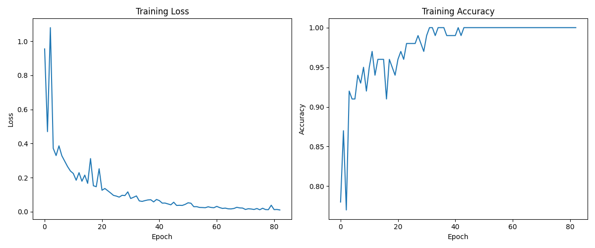
Figure 4: Training progress showing how loss decreases and accuracy improves as the model learns.

Our simple model learns to separate the two classes effectively, as shown by the decision boundary visualization in Figure 5:

Neural Network Decision Boundary
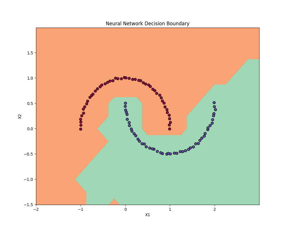
Figure 5: The learned decision boundary shows how our model separates the two classes with a non-linear boundary.

Optimization Opportunities

Neural network training presents numerous opportunities for parallelization across multiple dimensions. The most obvious is batch parallelism, where multiple training examples can be processed simultaneously through the network. Each example in a batch can be computed independently during the forward pass, and their gradients can be accumulated in parallel during backpropagation. Additionally, within each layer, matrix multiplications and element-wise operations can be parallelized across neurons and feature dimensions, creating a rich hierarchy of parallel computation that modern hardware can exploit.

This inherent parallelism modern GPUS ideal for deep learning workloads. Unlike CPUs, which are optimized for sequential processing with complex control flow, GPUs contain thousands of simpler cores designed specifically for parallel arithmetic operations. This architecture aligns perfectly with neural network computations—matrix multiplications, convolutions, and element-wise operations can all be distributed across these cores, leading to orders of magnitude speedup compared to CPU implementations. Modern GPUs also feature specialized tensor cores that accelerate mixed-precision matrix operations commonly found in deep learning.

The memory hierarchy of GPUs is another crucial factor in their deep learning performance. High-bandwidth memory and sophisticated caching mechanisms allow GPUs to feed data to their numerous processing cores efficiently, while shared memory enables fast communication between threads working on the same computation. This is particularly important for deep learning, where memory access patterns are predictable and regular, allowing for optimal utilization of the memory subsystem. Combined with their massive parallel processing capability, these memory characteristics make GPUs the backbone of modern deep learning infrastructure, enabling the training of increasingly large and complex models. We'll move onto that next.